Tutorial
This tutorial demonstrates the usage of the sweights package.
We will first cook up a toy model with a discriminat variable (invariant mass) and a control variable (decay time) and use it to generate some toy data.
Then we will use a fit to the invariant mass to obtain some component pdf estimates and use these to extract some weights which project out the signal only component in the decay time.
We will demonstrate both the classic sWeights and the Custom Ortogonal Weight functions (COWs) method. See arXiv:2112.04575 for more details.
Finally we will fit the weighted decay time distribution and correct the covariance matrix according to the description in arXiv:1911.01303.
[1]:
# external requirements
import os
import numpy as np
from scipy.stats import norm, expon, uniform
import matplotlib.pyplot as plt
from iminuit import Minuit
from iminuit.cost import ExtendedUnbinnedNLL
from iminuit.pdg_format import pdg_format
import boost_histogram as bh

# from this package
from sweights import SWeight # for classic sweights
from sweights import Cow     # for custom orthogonal weight functions
from sweights import cov_correct, approx_cov_correct # for covariance corrections
from sweights import kendall_tau # for an independence test
from sweights import plot_indep_scatter

# set a reproducible seed
np.random.seed(21011987)
Make the toy model and generate some data
[2]:
Ns = 5000
Nb = 5000
ypars = [Ns,Nb]

# mass
mrange = (0,1)
mu = 0.5
sg = 0.1
lb = 1
mpars = [mu,sg,lb]

# decay time
trange = (0,1)
tlb = 2
tpars = [tlb]

# generate the toy
def generate(Ns,Nb,mu,sg,lb,tlb,poisson=False,ret_true=False):

    Nsig = np.random.poisson(Ns) if poisson else Ns
    Nbkg = np.random.poisson(Nb) if poisson else Nb

    sigM = norm(mu,sg)
    bkgM = expon(mrange[0], lb)

    sigT = expon(trange[0], tlb)
    bkgT = uniform(trange[0],trange[1]-trange[0])

    # generate
    sigMflt = sigM.cdf(mrange)
    bkgMflt = bkgM.cdf(mrange)
    sigTflt = sigT.cdf(trange)
    bkgTflt = bkgT.cdf(trange)

    sigMvals = sigM.ppf( np.random.uniform(*sigMflt,size=Nsig) )
    sigTvals = sigT.ppf( np.random.uniform(*sigTflt,size=Nsig) )

    bkgMvals = bkgM.ppf( np.random.uniform(*bkgMflt,size=Nbkg) )
    bkgTvals = bkgT.ppf( np.random.uniform(*bkgTflt,size=Nbkg) )

    Mvals = np.concatenate( (sigMvals, bkgMvals) )
    Tvals = np.concatenate( (sigTvals, bkgTvals) )

    truth = np.concatenate( ( np.ones_like(sigMvals), np.zeros_like(bkgMvals) ) )

    if ret_true:
        return np.stack( (Mvals,Tvals,truth), axis=1 )
    else:
        return np.stack( (Mvals,Tvals), axis=1 )

toy = generate(Ns,Nb,mu,sg,lb,tlb,ret_true=True)
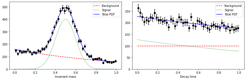
Plot the toy data and generating pdfs
[3]:
# useful function for plotting data points with error bars
def myerrorbar(data, ax, bins, range, wts=None, label=None, col=None):
    col = col or 'k'
    nh, xe = np.histogram(data,bins=bins,range=range)
    cx = 0.5*(xe[1:]+xe[:-1])
    err = nh**0.5
    if wts is not None:
        whist = bh.Histogram( bh.axis.Regular(bins,*range), storage=bh.storage.Weight() )
        whist.fill( data, weight = wts )
        cx = whist.axes[0].centers
        nh = whist.view().value
        err = whist.view().variance**0.5

    ax.errorbar(cx, nh, err, capsize=2,label=label,fmt=f'{col}o')

# define the mass pdf for plotting etc.
def mpdf(x, Ns, Nb, mu, sg, lb, comps=['sig','bkg']):

    sig  = norm(mu,sg)
    sigN = np.diff( sig.cdf(mrange) )

    bkg  = expon(mrange[0], lb)
    bkgN = np.diff( bkg.cdf(mrange) )

    tot = 0
    if 'sig' in comps: tot += Ns * sig.pdf(x) / sigN
    if 'bkg' in comps: tot += Nb * bkg.pdf(x) / bkgN

    return tot

# define time pdf for plotting etc.
def tpdf(x, Ns, Nb, tlb, comps=['sig','bkg']):

    sig  = expon(trange[0],tlb)
    sigN = np.diff( sig.cdf(trange) )

    bkg  = uniform(trange[0],trange[1]-trange[0])
    bkgN = np.diff( bkg.cdf(trange) )

    tot = 0
    if 'sig' in comps: tot += Ns * sig.pdf(x) / sigN
    if 'bkg' in comps: tot += Nb * bkg.pdf(x) / bkgN

    return tot

# define plot function
def plot(toy, draw_pdf=True):

    nbins = 50

    fig, ax = plt.subplots(1,2,figsize=(12,4))

    myerrorbar(toy[:,0],ax[0],bins=nbins,range=mrange)
    myerrorbar(toy[:,1],ax[1],bins=nbins,range=trange)

    if draw_pdf:
        m = np.linspace(*mrange,400)
        mN = (mrange[1]-mrange[0])/nbins

        bkgm = mpdf(m, *(ypars+mpars),comps=['bkg'])
        sigm = mpdf(m, *(ypars+mpars),comps=['sig'])
        totm = bkgm + sigm

        ax[0].plot(m, mN*bkgm, 'r--', label='Background')
        ax[0].plot(m, mN*sigm, 'g:' , label='Signal')
        ax[0].plot(m, mN*totm, 'b-' , label='Total PDF')

        t = np.linspace(*trange,400)
        tN = (trange[1]-trange[0])/nbins

        bkgt = tpdf(t, *(ypars+tpars),comps=['bkg'])
        sigt = tpdf(t, *(ypars+tpars),comps=['sig'])
        tott = bkgt + sigt

        ax[1].plot(t, tN*bkgt, 'r--', label='Background')
        ax[1].plot(t, tN*sigt, 'g:' , label='Signal')
        ax[1].plot(t, tN*tott, 'b-' , label='Total PDF')

    ax[0].set_xlabel('Invariant mass')
    ax[0].set_ylim(bottom=0)
    ax[0].legend()

    ax[1].set_xlabel('Decay time')
    ax[1].set_ylim(bottom=0)
    ax[1].legend()

    fig.tight_layout()

plot(toy)
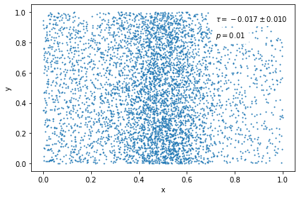
Check the independence of our data
By computing the kendall rank coefficient and seeing how compatibile it is with 0
[4]:
kts = kendall_tau(toy[:,0],toy[:,1])
print('Kendall Tau:', pdg_format( kts[0], kts[1] ) )
plot_indep_scatter(toy[:,0],toy[:,1],reduction_factor=2);
Kendall Tau: -0.017 ± 0.010
Fit the toy in invariant mass
This provides us with estimates for the component shapes and the component yields
[5]:
# define mass pdf for iminuit fitting
def mpdf_min(x, Ns, Nb, mu, sg, lb):
    return (Ns+Nb, mpdf(x, Ns, Nb, mu, sg, lb) )

mi = Minuit( ExtendedUnbinnedNLL(toy[:,0], mpdf_min), Ns=Ns, Nb=Nb, mu=mu, sg=sg, lb=lb )
mi.limits['Ns'] = (0,Ns+Nb)
mi.limits['Nb'] = (0,Ns+Nb)
mi.limits['mu'] = mrange
mi.limits['sg'] = (0,mrange[1]-mrange[0])
mi.limits['lb'] = (0,10)

mi.migrad()
mi.hesse()
display(mi) # only valid for ipython notebooks
| Migrad | ||||
|---|---|---|---|---|
| FCN = -1.684e+05 | Nfcn = 135 | |||
| EDM = 7.37e-05 (Goal: 0.0002) | ||||
| Valid Minimum | No Parameters at limit | |||
| Below EDM threshold (goal x 10) | Below call limit | |||
| Covariance | Hesse ok | Accurate | Pos. def. | Not forced |
| Name | Value | Hesse Error | Minos Error- | Minos Error+ | Limit- | Limit+ | Fixed | |
|---|---|---|---|---|---|---|---|---|
| 0 | Ns | 5.11e3 | 0.11e3 | 0 | 1E+04 | |||
| 1 | Nb | 4.89e3 | 0.11e3 | 0 | 1E+04 | |||
| 2 | mu | 0.4981 | 0.0021 | 0 | 1 | |||
| 3 | sg | 0.1031 | 0.0022 | 0 | 1 | |||
| 4 | lb | 1.07 | 0.06 | 0 | 10 |
| Ns | Nb | mu | sg | lb | |
|---|---|---|---|---|---|
| Ns | 1.22e+04 | -7.12e+03 (-0.587) | -0.00789 (-0.034) | 0.124 (0.516) | -1.44 (-0.203) |
| Nb | -7.12e+03 (-0.587) | 1.2e+04 | 0.00788 (0.034) | -0.124 (-0.520) | 1.44 (0.205) |
| mu | -0.00789 (-0.034) | 0.00788 (0.034) | 4.46e-06 | -2.09e-07 (-0.045) | -3.35e-05 (-0.247) |
| sg | 0.124 (0.516) | -0.124 (-0.520) | -2.09e-07 (-0.045) | 4.72e-06 | -2.39e-05 (-0.172) |
| lb | -1.44 (-0.203) | 1.44 (0.205) | -3.35e-05 (-0.247) | -2.39e-05 (-0.172) | 0.00411 |
Construct the sweighter
Note that this will run much quicker if verbose=False and checks=False
[6]:
# define estimated functions
spdf = lambda m: mpdf(m,*mi.values,comps=['sig'])
bpdf = lambda m: mpdf(m,*mi.values,comps=['bkg'])

# make the sweighter
sweighter = SWeight( toy[:,0], [spdf,bpdf], [mi.values['Ns'],mi.values['Nb']], (mrange,), method='summation', compnames=('sig','bkg'), verbose=True, checks=True )
Initialising sweight with the summation method:
    PDF normalisations:
         0 5107.224408977729
         1 4892.156810093505
    W-matrix:
        [[1.38699027e-04 5.96207082e-05]
         [5.96207082e-05 1.42184207e-04]]
    A-matrix:
        [[ 8795.16287156 -3687.98933236]
         [-3687.98933236  8579.57828096]]
    Integral of w*pdf matrix (should be close to the
                identity):
        [[ 1.00011709e+00 -1.32635071e-04]
         [-1.57992838e-04  1.00004886e+00]]
    Check of weight sums (should match yields):
        Component  | sWeightSum |   Yield    |   Diff    |
        ---------------------------------------------------
          0        |  5107.2244 |  5107.2244 |    -0.00% |
          1        |  4892.1568 |  4892.1568 |     0.00% |
Construct the COW
Note that COW pdfs are always normalised in the COW numerator so that the W and A matrices tend to come out with elements of order one. This example uses a variance function of unity, I(m)=1, but also codes the case where I(m) = g(m), which is equiavalent to sweights.
[7]:
# unity
Im = 1
# sweight equiavlent
# Im = lambda m: mpdf(m,*mi.values) / (mi.values['Ns'] + mi.values['Nb'] )

# make the cow
cw = Cow(mrange, spdf, bpdf, Im, verbose=True)
Initialising COW:
    W-matrix:
        [[2.73492037 0.97050271]
          [0.97050271 1.07239023]]
    A-matrix:
        [[ 0.53861176 -0.48743839]
          [-0.48743839  1.37362336]]
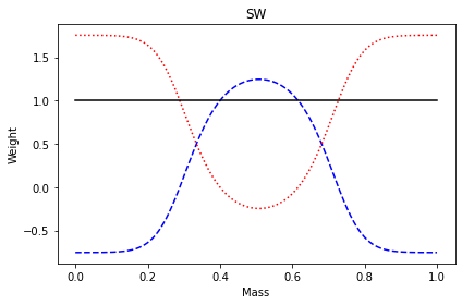
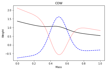
Comparison of the sweight and COW methods
Compare the weight distributoins
[8]:
def plot_wts(x, sw, bw, title=None):
    fig,ax = plt.subplots()
    ax.plot(x, sw, 'b--', label='Signal')
    ax.plot(x, bw, 'r:' , label='Background')
    ax.plot(x, sw+bw, 'k-', label='Sum')
    ax.set_xlabel('Mass')
    ax.set_ylabel('Weight')
    if title: ax.set_title(title)
    fig.tight_layout()

for meth, cls in zip( ['SW','COW'], [sweighter,cw] ):

    # plot weights
    x = np.linspace(*mrange,400)
    swp = cls.get_weight(0,x)
    bwp = cls.get_weight(1,x)
    plot_wts(x, swp, bwp, meth)
Fit the weighted data in decay time and correct the covariance
[9]:
# define weighted nll
def wnll(tlb, tdata, wts):
    sig  = expon(trange[0],tlb)
    sigN = np.diff( sig.cdf(trange) )
    return -np.sum( wts * np.log( sig.pdf( tdata ) / sigN ) )

# define signal only time pdf for cov corrector
def tpdf_cor(x, tlb):
    return tpdf(x,1,0,tlb,['sig'])

flbs=[]
for meth, cls in zip( ['SW','COW'], [sweighter,cw] ):

    print('Method:', meth)
    # get the weights
    wts = cls.get_weight(0,toy[:,0])

    # define the nll
    nll = lambda tlb: wnll(tlb, toy[:,1], wts)

    # do the minimisation
    tmi = Minuit( nll, tlb=tlb )
    tmi.limits['tlb'] = (1,3)
    tmi.errordef = Minuit.LIKELIHOOD
    tmi.migrad()
    tmi.hesse()

    # and do the correction
    fval = np.array(tmi.values)
    flbs.append(fval[0])
    fcov = np.array( tmi.covariance.tolist() )

    # first order correction
    ncov = approx_cov_correct(tpdf_cor, toy[:,1], wts, fval, fcov, verbose=False)

    # second order correction
    hs  = tpdf_cor
    ws  = lambda m: cls.get_weight(0,m)
    W   = cls.Wkl

    # these derivatives can be done numerically but for the sweights / COW case it's straightfoward to compute them
    ws = lambda Wss, Wsb, Wbb, gs, gb: (Wbb*gs - Wsb*gb) / ((Wbb-Wsb)*gs + (Wss-Wsb)*gb)
    dws_Wss = lambda Wss, Wsb, Wbb, gs, gb: gb * ( Wsb*gb - Wbb*gs ) / (-Wss*gb + Wsb*gs + Wsb*gb - Wbb*gs)**2
    dws_Wsb = lambda Wss, Wsb, Wbb, gs, gb: ( Wbb*gs**2 - Wss*gb**2 ) / (Wss*gb - Wsb*gs - Wsb*gb + Wbb*gs)**2
    dws_Wbb = lambda Wss, Wsb, Wbb, gs, gb: gs * ( Wss*gb - Wsb*gs ) / (-Wss*gb + Wsb*gs + Wsb*gb - Wbb*gs)**2

    tcov = cov_correct(hs, [spdf,bpdf], toy[:,1], toy[:,0], wts, [mi.values['Ns'],mi.values['Nb']], fval, fcov, [dws_Wss,dws_Wsb,dws_Wbb],[W[0,0],W[0,1],W[1,1]], verbose=False)
    print('Method:', meth, f'- covariance corrected {fval[0]:.2f} +/- {fcov[0,0]**0.5:.2f} ---> {fval[0]:.2f} +/- {tcov[0,0]**0.5:.2f}')
Method: SW
Method: SW - covariance corrected 1.71 +/- 0.14 ---> 1.71 +/- 0.19
Method: COW
Method: COW - covariance corrected 1.64 +/- 0.13 ---> 1.64 +/- 0.18
[10]:
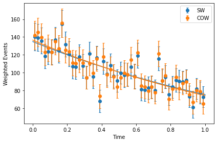
### Plot the weighted decay distributions and the fit result
def plot_tweighted(x, wts, wtnames=[], funcs=[]):

    fig, ax = plt.subplots()

    t = np.linspace(*trange,400)
    N = (trange[1]-trange[0])/50

    for i, wt in enumerate(wts):
        label = None
        if i<len(wtnames): label = wtnames[i]
        myerrorbar(x, ax, bins=50, range=trange, wts=wt, label=label, col=f'C{i}')
        if i<len(funcs):
            ax.plot(t,N*funcs[i](t),f'C{i}-')

    ax.legend()
    ax.set_xlabel('Time')
    ax.set_ylabel('Weighted Events')
    fig.tight_layout()

swf  = lambda t: tpdf(t, mi.values['Ns'], 0, flbs[0], comps=['sig'] )
cowf = lambda t: tpdf(t, mi.values['Ns'], 0, flbs[1], comps=['sig'] )
sws  = sweighter.get_weight(0, toy[:,0])
scow = cw.get_weight(0, toy[:,0])

plot_tweighted(toy[:,1], [sws,scow], ['SW','COW'], funcs=[swf,cowf] )
Write the weights back into a file
For example into a pandas dataframe or root file
[11]:
import pandas as pd

df = pd.DataFrame( )
df['mass'] = toy[:,0]
df['time'] = toy[:,1]
df['sw_sws'] = sweighter.get_weight(0, df['mass'].to_numpy() )
df['sw_bws'] = sweighter.get_weight(1, df['mass'].to_numpy() )
df['cow_sws'] = cw.get_weight(0, df['mass'].to_numpy() )
df['cow_bws'] = cw.get_weight(1, df['mass'].to_numpy() )

import uproot

with uproot.recreate('outf.root') as f:
    f['tree'] = df

print(df)
          mass      time    sw_sws    sw_bws   cow_sws   cow_bws
0     0.276401  0.287028 -0.129313  1.129223 -0.372759  1.446466
1     0.302426  0.426394  0.150924  0.848999 -0.220921  1.282285
2     0.578586  0.449921  1.149476 -0.149511  1.099331 -0.159718
3     0.373953  0.741222  0.839109  0.160843  0.481153  0.576620
4     0.515549  0.598659  1.244910 -0.244940  1.590285 -0.553110
...        ...       ...       ...       ...       ...       ...
9995  0.846222  0.426296 -0.706615  1.706501 -0.332575  0.950587
9996  0.166248  0.153495 -0.711678  1.711563 -0.631136  1.801133
9997  0.535665  0.266288  1.231984 -0.232015  1.494705 -0.483188
9998  0.357202  0.365763  0.708016  0.291931  0.282588  0.772361
9999  0.643105  0.593656  0.832079  0.167873  0.364086  0.456587

[10000 rows x 6 columns]